Brownian Motion

Geometric Brownian Motion (GBM) is an ubiquitous random process, used not only in science, but also in finance, for example in the Black-Scholes model. First of all, we need to specify what we mean with Geometric Brownian Motion. As the name suggests, the main ingredient of such mathematical object is the Brownian Motion, a continuous-time random process that can be thought of as the limit of a Random Walk. The other ingredients that we need are a mean value, $\mu$, and a variance, $\sigma^2$, representing the “volatility” of variable that we are modeling.

We generate our Brownian motion, $W$ starting from a Random Walk. It’s worth mentioning some fundamental facts:

1. $W_0 = 0$.
2. $W$ is made of stationary and independent increments.
3. $W_t - W_s$ is normally distributed with mean 0 and variance $t-s$, for $0\leq s < t$,

so that $(W_{t_i} - W_{t_{i-1}}) \sim \mathcal{N}(0, t_i - t_{i-1})$. Considering that a normal variable $\sim \mathcal{N}_t(0,\sigma^2)$ can be represented as $\sim \sigma \mathcal{N}_t(0,1)$. Take a standard normal variable $\epsilon_i$. Considering property 3 from the list above, we can simulate our brownian motion by generating increments

that is, we calculate the increments of the Brownian motion as being $\sqrt{dt}$ times a standard normal variable, which is easy to generate in Python. We have assumed $t_i - t_{i-1} = dt\; \forall i.$ In practice what we’re saying is that $W_{t_1} = \sqrt{t_1} Z_1, W_{t_2} = W_{t_1} + \sqrt{t_2 - t_1} Z_1, \ldots, W_{t_n} = \sqrt{dt}\sum\limits_i^n Z_i,$, where $Z_i$ is a standard normal variable. in the Python code below, we’re calculating $W_{t_n}$ as we have just described, the relevant variable is called “W”.

In a Brownian Motion with Drift $\mu$ we have instead \begin{equation} W_{t_n} = \sum\limits_i^n\sqrt{dt}\;\epsilon_i + dt\;\mu. \end{equation}

Geometric Brownian Motion

The final step is to calcualte the Geometric Brownian Motion \begin{equation} S_t = S_0 \exp\bigg(\big(\mu - \dfrac{\sigma^2}{2}\big)t + \sigma W_t\bigg), \end{equation}

which is implemented in line 41 in the code below. To make a practical example, I will get the values for the mean $\mu$ and the volatility $\sigma^2$ from the close prices of EURUSD. Moreover We assume that the close prices are normally distributed (more below) and perform a Maximum Likelihood Estimation as well as a Kernel Density Estimation (KDE) on the EURUSD returns. Notice that the results are in $10^{-4}$ pips, thus the small numbers for $\mu$ and $\sigma$. We have all the ingredients to generate our GBMs. Time to write some code!

import numpy as np
import scipy.stats as stats
import matplotlib.pyplot as plt
import matplotlib
import pandas as pd


matplotlib.rcParams.update({'font.size': 18})

# EURUSD close prices
data = pd.read_csv('data.csv', delimiter=';', engine='c', nrows=1000)
close = []
for dataIter in data.iterrows():
    close.append(dataIter[1][4])

# work with retuns
ret = np.diff(close)
ln = len(ret)
x = np.linspace(min(ret), max(ret), ln)
# time "normalized" between 0 and 1
t = np.linspace(0, 1, ln)
# time step
dt = t/ln
# n_samp samples from the GBM process
n_samp = 15

# MLE returns to calculate mu and sigma and calculate the pdf
mu, sigma = stats.norm.fit(ret)
norm = stats.norm.pdf(x, loc=mu, scale=sigma)
# Kernel Density Estimation
kernel = stats.gaussian_kde(ret)
ker = kernel(x)

# Sample the process
W = np.empty((ln, n_samp))
gbm = np.empty((ln, n_samp))

for i in range(n_samp):    
    # random walk variates "W" from standard normal, "drive" the GBM process called "gbm"
    W[:, i] = np.hstack(np.sqrt(dt) * np.cumsum( stats.norm.rvs(loc=0, scale=1, size=ln)))  
    gbm[:, i] = close[0] * np.exp((mu - 0.5 * sigma**2) * t + sigma * W[:, i])
    # gbm[:, i] = close[0] * np.exp((.1 - 0.5 * 0.2**2) * t + 2 * W[:, i])  # mu = 0.1, sigma = 0.2

fig, ax = plt.subplots(2, 1, figsize=(17, 10))

ax[0].plot(x, ker, label='Kernel Estimate', linewidth=3 )
plt_str = "$\mathcal{N}$"+"({0:4.3E}, {1:4.2E})".format(mu, sigma)
ax[0].plot(x, norm, label=plt_str, linewidth=3)
ax[0].hist(ret, bins=30, normed=True, label='Histogram')
ax[0].set_xlim([min(x), max(x)])
ax[0].legend()

ax[1].plot(t, gbm, label=gbm)
ax[1].set_title("Geometric Brownian " + "($\mu$ = {0:4.3E}, $\sigma$ = {1:4.2E})".format(mu, sigma))
ax[1].set_xlabel("normalized time")
ax[1].set_ylabel("GBM($\mu$=0, $\sigma$=1)")

plt.tight_layout(pad=0.4, w_pad=0.5, h_pad=1.0)
ax[1].set_xlim([0, 1])

plt.show()

The code is quite self-explanatory. First we load the data. We then define the returns and calculate the mean and volatility of the EURUSD close prices. Finally we calculate (15 = nsamp) possible realization of the Wiener process needed to compute the GBM (lines 40 and 41).

Example: Option Pricing

There are good introductions on the web about the Black-Scholes-Merton (BSM) model, as well as good books. I suggest for example the books Arbitrage Theory in Continuous Time and Stochastic Calculus for Finance II . Here I propose an example that allows to understand at a glance what we’re talking about

The Black-Scholes-Merton model is an option pricing model, that is, it gives the price of a contract as function of the price of the underlying. In this sense it is not an absolute measure of the price of the contract. It can be shown that in an arbitrage-free market, the price of the option has to follow the BSM equation.

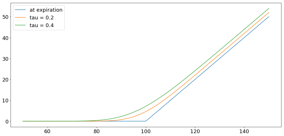
There are a few contracts for which the solution of the BSM equation is known. Different contracts imply a different price at maturity, that is, a different boundary conditions. A tractable case is the pricing of a call option contract. In the risk-neutral measure we compute the value of the call option solving BSM equation analytically. The Price of the call option is

\begin{equation} F(t,s) = s\,N[d_+(t,s)] - \exp^{-r\,(t-T)}\,K\,N[d_-(t,s)] \end{equation} with \begin{equation} d_{\pm}(t,s) = \dfrac{1}{\sigma\sqrt{T - t}}\bigg[ \ln\bigg(\dfrac{s}{K}\bigg) + \big( r \pm \dfrac{\sigma^2}{2}\big)\,(T-t) \bigg] \end{equation}

where, $s$ is the current price of the underlying, $T$ is the expiration date, $K$ is the strike price, $r$ is the interest rate and $\sigma$ is the volatility.

The quantity $F(t,s)$ measures the value of the option contract at time $t$ for the underlying with price $s$.

Let’s make an example. Mantaining the code above we jsut need to change the value of the volatility and add the following code. Here, tau $= T-t$.

# BSM Model
s = np.linspace(50, 150, 1000)

tau = np.array([0.0001, 0.2, 0.4])
K = 100
r = 0.1
sigma = 0.2

F = np.zeros((len(s), len(tau)))
for i in range(0, len(tau)):
    d1 = (1/(sigma * np.sqrt(tau[i]))) * (np.log(s/K) + (r + 0.5 * sigma**2) * tau[i])
    d2 = (1/(sigma * np.sqrt(tau[i]))) * (np.log(s/K) + (r - 0.5 * sigma**2) * tau[i])
    F[:, i] = s * stats.norm.cdf(d1) - K * np.exp(-r * tau[i]) * stats.norm.cdf(d2)

plt.figure(figsize=(17,8))
plt.plot(s, F[:,0], label='at expiration')
plt.plot(s, F[:,1], label="tau = 0.2")
plt.plot(s, F[:,2], label="tau = 0.4")
plt.legend(loc='upper left')
plt.show()

Calls and Puts, Buy and Sell

Coming soon!