Support Vector Machines, Kernels and Hilbert Spaces

In a classification problem we want to classify or label a new observation, having trained our model with a set of observations whose class is known. One approach is to think that all elements that belong to the same class are similar in some way. We thus need a concept of similarity or distance.

For example, if we had to classify cars, we could choose some fundamental features, such as weight, engine power and mileage. Having a list of cars with such information divided in two parts, good cars and bad cars, can we classify the next car we come across as being part of the group of good cars or bad cars?

We need a model to distinguish the good cars from the bad ones. How does the model do that? First of all we train our model on a known set of good and bad cars. Then, we need a concept of distance to compare the features of the good (bad) cars to the features of the next car we come across. Our concept of distance can’t really tell us if two cars (or two documents, or two audio files…) are distant, but it tells us if features are distant. If the distance between the features of the good (bad) cars and the car under observation is small, we are quite sure that the car is good (bad).

A Few Mathematical Details

There is plenty of material on books and internet about the background theory. I’m just giving a hint to fix some concepts, after all, this is a gentle introduction. Feel free to skip this section if you’re more example oriented. Those really intrested in (the very intresting) theory can check the literature. I recommend the book written by Kevin P. Murphy. Other resources are right here and here . The last reference is a paper by N. Aronszajn entitled “Theory of Reproducing Kernels”.

Reproducing Kernel Hilbert Space

We start with two fundamental steps

1. Let’s consider a bounded functional over the Hilbert space $\mathcal{H}$ of functions $f$, that is, $\mathcal{L}_x:f \rightarrow f(x)$. Notice that the functional $\mathcal{L}_x$ is somehow special, it evaluates the function at point $x$.
2. If the evaluation is bounded, that is if $\mathcal{L}_x$ is a continuous functional $\forall x\in\mathcal{X}$, then $\mathcal{H}$ is a reproducing kernel Hilbert space (RKHS) by definition.

Thanks to Riesz theorem, we know that bounded linear functionals defined in a Hilbert space $\mathcal{H}$, can be represented in a unique way with the inner product in $\mathcal{H}$, that is, $\forall f \in \mathcal{H}$ there is a unique $\kappa_x=\kappa(\cdot, x) \in \mathcal{H}, \forall x \in \mathcal{X}$, such that $\mathcal{L}[f]=\langle f,\kappa_x\rangle_H$, where the brackets represent the inner product in $\mathcal{H}$.

We now ask $\kappa_x$ to have the fundamental reproducing property \begin{equation} \forall x \in \mathcal{X},\forall f\in\mathcal{H},\;\;\langle f,\kappa(\cdot, x) \rangle_{\mathcal{H}} = f(x). \end{equation} Such $\kappa_x$ is the reproducing kernel of the Hilbert space $\mathcal{H}$. As the name suggests, it allows us to “evaluate” $f$ at $x$, $f$ being the “input” function and $f(x)$ being the output of the inner product. It is made of two “ingredients”, the reproducing property above, and the fact that $\kappa(\cdot, x) \in \mathcal{H}, \forall x \in \mathcal{X}$.

Since $\kappa(\cdot, x)\in \mathcal{H}, \forall x\in\mathcal{X}$, we can exploit the reproducing property and write that, $\forall x, y\in \mathcal{X}$ \begin{equation} \kappa(x,y)=\langle \kappa(\cdot, x), \kappa(\cdot, y)\rangle_{\mathcal{H}}. \end{equation}

Recap

So far we have defined the RKHS as a Hilbert space with funcionals that “reproduce” a function $f$ in a continuous way. We then went on to characterize such functionals. Thanks to Reisz theorem we represent such functionals in a unique way with the inner product in $\mathcal{H}$, which led us to define the reproducing kernel, $\kappa:\mathcal{X}\times\mathcal{X}\rightarrow\mathbb{R}$.

Thus, given a RKHS $\mathcal{H}$, we can define a reproducing kernel $\kappa$ associated with $\mathcal{H}$. Moreover, such kernel is unique and positive definite. The positive definiteness means that the matrix $\mathbf{K}$ with elements $K_{i,j}=\kappa(x_i,x_j)$, is positive definite. The uniqueness implies the fundamental fact that a Hilbert space $\mathcal{H}$ is a RKHS if and only if it has a reproducing kernel. We will use this below.

Features

Instead of starting from RKHSs, we can adopt another point of view and start from the definition of kernel. The function $\kappa:\mathcal{X}\times\mathcal{X}\rightarrow \mathbb{R}$ is a kernel if there exists a Hilbert space $\mathcal{H}$ and a feature map, $\phi(x):\mathcal{X}\rightarrow\mathcal{H},$ such that, $\forall x,y\in\mathcal{X}:$

\begin{equation} \kappa(x,y)=\langle \phi(x),\phi(y) \rangle_{\mathcal{H}}. \end{equation}

Such kernel is necessarily positive definite, thanks to the positive definiteness property of the inner product in $\mathcal{H}$. Furthermore, thanks to the Moore-Aronszajn (M-A) theorem, to every positive definite kernel there corresponds one and only one class of functions $f$ that forms a Hilbert space admitting $\kappa$ as a reproducing kernel. To summarize:

Given a RKHS, $\mathcal{H}$ $\Rightarrow$ it is possible to define the unique (Riesz Thm.) reproducing kernel with the inner product in $\mathcal{H}$

$\forall$ positive definite kernel $\Rightarrow$ (M-A thm.) it is a reproducing kernel $\Rightarrow$ (remember the “if and only if” above) there is a unique RKHS with $\kappa$ being its reproducing kernel.

Kernels practically

In general, we have objects $x$, belonging to a space $\mathcal{X}$. Our concept of similarity is embodied by a function $\mathcal{X}\times\mathcal{X}\rightarrow\mathbb{R}$ that we call Kernel Function. It is a measure of the distance between $x$ and $y$. It is natural to choose a kernel that is symmetric ($κ(x,y)=κ(y,x)κ(x,y)=κ(y,x)$), that is, the similarity or distance between $x$ and $y$ is the same as the distance between $y$ and $x$.

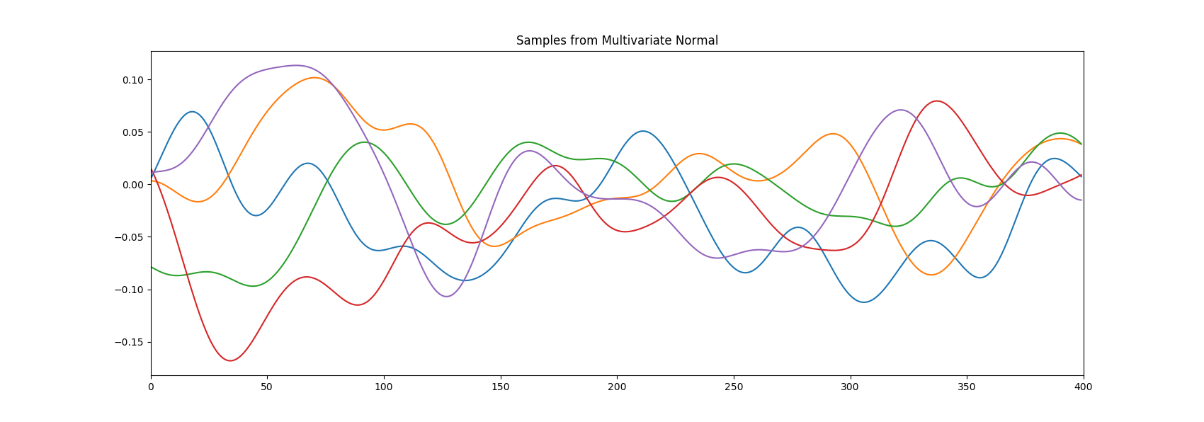
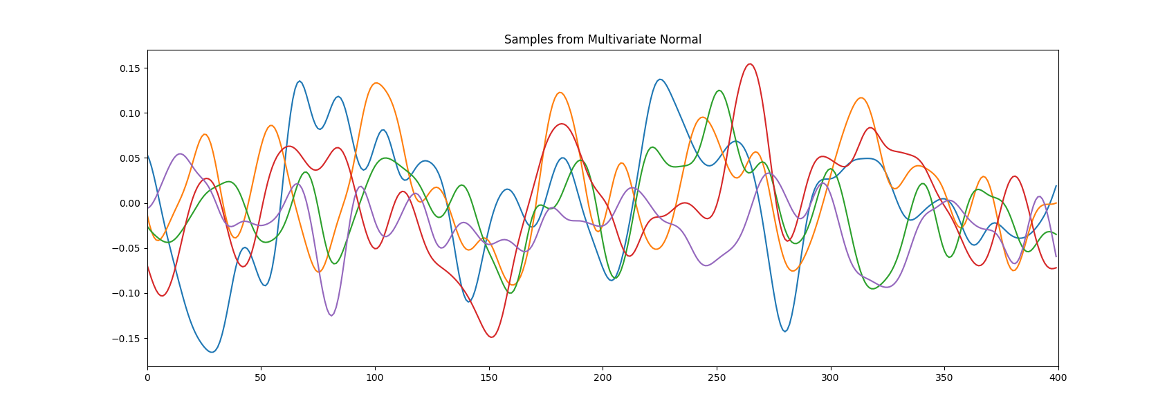
Two popular choices are the Gaussian kernel, \begin{equation} \kappa(x,x′) = \exp\bigg(−\dfrac{1}{2}(x−x′)^T\,\Sigma^{−1}\,(x−x′)\bigg), \end{equation} and the squared exponential, radial basis function (RBF), \begin{equation} \kappa(x,x′) = \exp\bigg(−\dfrac{||x−x′||}2{\sigma^2}\bigg). \end{equation} Of course there are many different kernels for different uses. Another choice worth mentioning is the Matern Kernel. Notice in the last formula how the parameter $\sigma$ influences the smoothness of the kernel. In other words, $\sigma$ controls how far away points “influence” our current point. if it is large, we allow points far away from the current point to be “taken into account” (correlate). If it is small, only points close to the current point will count.

Let’s make an example where we draw samples from a gaussian process with the squared exponential kernel. Don’t worry about the gaussian process part for now. In the first picture $\sigma=5$ while in the second $\sigma=2$. The difference in the smoothness of the curves is clear.

import numpy as np
import matplotlib.pyplot as plt

sample_size = 400
x_test = np.linspace(-50, 50, sample_size)


def kernel_fun(x, y, L, s):
    """ Computes the kernel function for two points x and y. """
    return (s ** 2) * np.exp(-(1.0 / (2 * L ** 2)) * abs(x - y) ** 2)


def kernel_matrix(x1, x2, L, s):
    """ Computes the kernel matrix. It's symmetric. """
    h = 1
    K = np.zeros((sample_size, sample_size))
    for i in xrange(0, sample_size):
        for j in xrange(0, h):  # fill the j-th column
            K[i][j] = kernel_fun(x1[i], x2[j], L, s)
        h = h + 1
    triu = np.triu_indices(sample_size)
    K[triu] = K.T[triu]
    return K
 
# Alternative with list comprehension
# def kernel_matrix(x1, x2, L, s):
#    return [[kernel_fun(v, w, L, s) for v in x1] for w in x2]
    
    
K2 = kernel_matrix(np.asarray(x_test), np.asarray(x_test), 2, .05)
K6 = kernel_matrix(np.asarray(x_test), np.asarray(x_test), 5, .05)


# Sample from the multivariate normal process with mean zero and cov=K
gauss_samples2 = np.random.multivariate_normal(np.zeros((sample_size, 1)).ravel(), K2, size=5)
gauss_samples5 = np.random.multivariate_normal(np.zeros((sample_size, 1)).ravel(), K6, size=5)

plt.figure(figsize=(17, 6))
plt.plot(gauss_samples2.T)
plt.title("Samples from Multivariate Normal")
plt.xlim([0, sample_size])
plt.figure(figsize=(17, 6))
plt.plot(gauss_samples5.T)
plt.title("Samples from Multivariate Normal")
plt.xlim([0, sample_size])
plt.show()

Decisions. Optimal Separating Hyperplane

Let’s put the pieces together. Consider the feature vector with n elements/features: $\Phi(x)=[x_1,x_2,x_3,…,x_n]$. If we were classifying cars, for example, the features could be, car weight, year of production, engine power. Cars could be hard to classify based on these features. What if we add another feature, that is, increase the dimension of the feature space? This feature doesn’t even have to be real, it’s used to increase the discriminative power of our algorithm since the features that we have are “insufficient”, i.e. our data looks like figure 1 below.

import numpy as np
import random
import matplotlib.pyplot as plt
from mpl_toolkits.mplot3d import Axes3D

N = 10
x1 = np.random.uniform(0, 2, N)
x2 = np.random.uniform(0, 3, N)

plt.figure()
plt.plot(x1, x2, '.b')
plt.plot(2,3,'.r')
plt.xlabel('x1')
plt.ylabel('x2')
plt.title('Figure 1')
plt.show()

# What if we add a feature?
x3 = np.hstack((np.zeros(N/2), np.ones(N/2)))

fig = plt.figure()
ax = Axes3D(fig)
ax.scatter(x1, x2, x3, c='b')
ax.scatter(2,3,1,c='r')  # Plot a red point for reference
# Plot a surface
# p = fig.gca()
# X, Y = np.meshgrid(np.arange(0, 1, 0.1) * 2, np.arange(0, 1, 0.1) * 3)
# p.plot_surface(X, Y, np.ones((N,N)) * 0.5, alpha=0.2)
ax.set_xlabel('x1')
ax.set_ylabel('x2')
ax.set_zlabel('x3')
ax.set_title('Figure 2')
# ax.azim = 80
ax.elev = 70
plt.show()

fig = plt.figure()
ax = Axes3D(fig)
ax.scatter(x1, x2, x3, c='b')
ax.scatter(2,3,1,c='r')
# Plot a surface
p = fig.gca()
X, Y = np.meshgrid(np.arange(0, 1, 0.1) * 2, np.arange(0, 1, 0.1) * 3)
p.plot_surface(X, Y, np.ones((N,N)) * 0.5, alpha=0.2)
ax.set_xlabel('x1')
ax.set_ylabel('x2')
ax.set_zlabel('x3')
ax.set_title('Figure 3')
# ax.azim = 80
ax.elev = 30
plt.show()

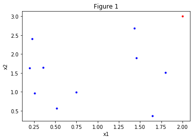
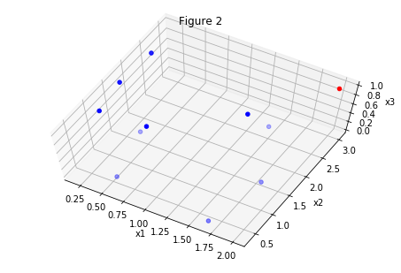
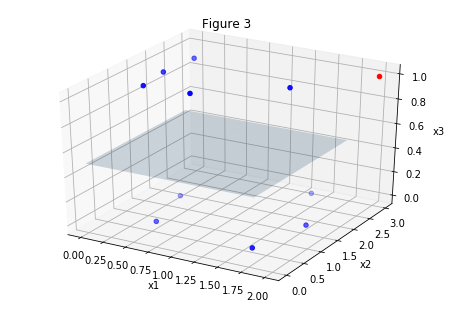
The same set of points is plotted in the figures above. In figure 1 we are looking at the dataset “from above”. Figures 2 and 3 are the “tilted” version of figure 1, but we have added a feature, the third dimension. Now it’s easy to classify points, look there is even a plane clearly dividing the set in two!

Is this the solution to all our classification problems? No unfortunately. If we add too many dimensions, we seriously risk to overfit our data.

Down to Business

As mentioned, support vector machines (SVMs) allow us to solve classification problems (as well as regression problems in fact). If we have a set of points, and two labels , for example 0 and 1 (or good, bad), we want to label the next observed point as being a 0 or a 1.

Linear SVMs separate the input data by finding an hyperplane between them such that the orthogonal distance between the plane and the closest point is maximized. Almost like in figure 3 above, but better, in an optimal, algorithmic way. Non Linear SVMs find non linear boundaries to separate subsets of points into classes (our labels).

The problem of finding such hyperplane (or hypersurface in the non linear case) in an optimal way can be solved by optimization methods. One possibility is to fomalize the optimization as quadratic problem. This is a separate topic, discussing such algorithms would take us very far, so we defer the discussion (hopefully) to future posts.

From a practicap perspective, the main ingredients that we need are the labeled dataset to train the SVM, a kernel and an optimization method. We can use well established python modules for our SVMs.

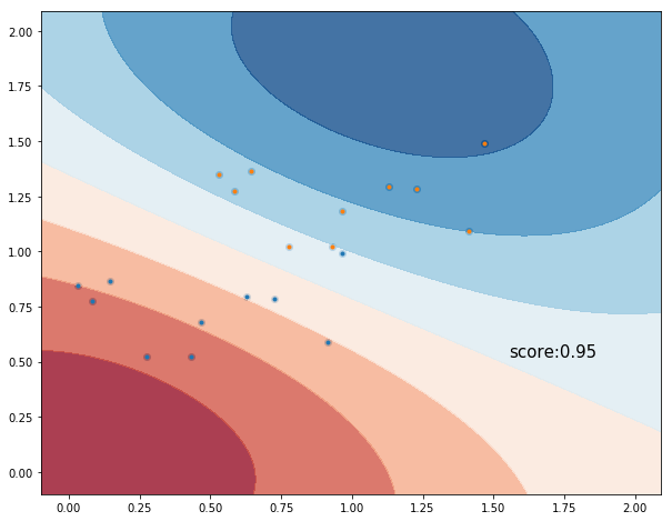
Example 1. Dual Label Classification

More explainations soon! For now here’s a worked out example. We classify two sets of points uniformly distributed and labeled with labels ‘a’ and ‘b’.

import numpy as np
import matplotlib.pyplot as plt
from sklearn import svm


# generate some data
feature1 = np.random.random((10, 2))
feature2 = feature1 + 0.5

plt.figure(figsize=(10,8))
plt.plot(feature1[:, 0], feature1[:, 1], '.')
plt.plot(feature2[:, 0], feature2[:, 1], '.')

# input data. rows are the "observations", columns are the features
x = np.hstack((feature1[:, 0], feature2[:, 0]))
y = np.hstack((feature1[:, 1], feature2[:, 1]))
dataset = np.vstack((x, y)).T

# generate the labels. Let's assume we have 3 labels. Can be strings or integers.
# Let's say the 1/2 of our data is labeled 'a,', another 1/2 is 'b'
labela = ['a'] * 10
labelb = ['b'] * 10

labels = labela + labelb

# define the SVM
classifier = svm.SVC()
classifier.fit(dataset, labels)
score = classifier.score(dataset, labels)

plt.scatter(dataset[:, 0], dataset[:, 1])

X, Y = np.meshgrid(np.arange(-.1, 2.1, .01), np.arange(-.1, 2.1, .01))
Z = classifier.decision_function(np.c_[X.ravel(), Y.ravel()])

Z = Z.reshape(X.shape)
plt.contourf(X, Y, Z, cmap=plt.cm.RdBu, alpha=.8)
plt.text(dataset[:, 0].max() + 0.4, dataset[:, 1].min(), ('score:' + '%.2f' % score).lstrip('0'),
         size=15, horizontalalignment='right')
plt.show()

Example 2. Multi-label Classification

Coming Soon!