Support Vector Machines, a Gentle Introduction

Classification in the Linear Case

Consider a set of points $\{x\}_i$ which constitute our observations or test set. These points labeled (or classified) as 1 or -1, see figure 1. The blue points are classified as -1 and the green points as 1. Formally we write that the class/label of the generic point $x_i$ is $y_i\in\{-1,1\}$ . If we had a new observation point $x_k$ (in red in figure 1),

how would we classify it? Should we choose $y_k = -1$ or $y_k=1$ ?
How to quantify the confidence we have that the point belongs to that class?

This is a Classification Problem. The training set is made of points $(\mathbf{x}_i,y_i)$ where $\mathbf{x}_i\in\mathbb{R}^n$ , and we want to learn the mapping $\mathbf{x}_i\mapsto y_i$ .

png

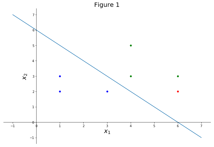
Figure 1. The third axis $x_3$ is perpendicular with respect to $x_1$ and $x_2$ , that is “coming out” of the screen/paper. The blue “line” is in fact a plane.

Functional and Geometric margin

A simple solution would be to draw a plane (hyperplane in higher dimensional spaces) that separates the points in some optimal way. We take all our observation points (test set) and draw a separating plane so that on one side we have observations with one label and on the other side we have observation with the other label. The optimality is in the fact that we require the points on the two sides to be as far as possible from the separating plane. In the plot above we have all the points below the plane in the class -1, and the points above the plane in the class +1.

It won’t always be easy to separate exactly the points, some points with one label may end up on the wrong side! As long as most points are well classified the classification is ok. We can still get an “optimal” solution to our ploblem, the perfect one is hard to achieve. So it’s not necessarily a problem if your test set is hard to separate “perfectly”.

Now that we have an idea on how to procede, we can try to answer question nr. 1. Intuitively we could write a function that assumes positive values for correctly classified points and negative values for incorrectly classified points. We could give observations as input and obtain a poisitive or negative number as output if the point is correctly or incorrectly classified, respectively. Moreover we could ask that function to assume higher (absolute) values the higher our confidence in the ownership of the input point to the predicted class…makes sense.

Functional Margin

We choose this function to be similar to the equation of an hyperplane (line in 2D). A plane in 3D (or higher dimension) is the set of points that satisfies

\begin{equation} a\,(x_1-x_{10}) + b\,(x_2-x_{20}) + c\,(x_3-x_{30})=0 \;\;\;\;\text{or}\;\;\;\;\; a\,x_1 + b\,x_2 + c\,x_3 + d = 0 \end{equation}

with $d = -(a\,x_{10} + b\,x_{20} + c\,x_{30})$ . We can rewrite the formula above with an inner product:

\begin{equation} \mathbf{w}\cdot \mathbf{x} + d = 0,\;\;\mathbf{w} = (a,b,c),\;\;\mathbf{x} = (x_1, x_2, x_3). \end{equation}

where $\cdot$ is the dot product between vectors (we write $\mathbf{\alpha}^T\mathbf{\beta}$ simply as $\mathbf{\alpha}\cdot\mathbf{\beta}$ , i.e. the transposition is understood). The plane in the figure above has $\mathbf{w} = (1, 1, 0)$ and $d = -6$ . The candidate function that we are looking for could be the funcitonal margin, which is

\begin{equation} \gamma = y_i (\mathbf{w}\cdot\mathbf{x} + d). \end{equation}

Let’s try it out. Consider the point $\mathbf{x} = (1, 2, 0)$ , classified as $y=-1$ (see figure 1 above). We have $\gamma = -1\big((1, 1) \cdot (1, 2, 0) - 6 \big) = 3 > 0$ . That is correct, $\gamma > 0$ for correctly classified points and $\mathbf{x} = (1, 2, 0)$ is in fact classified as $-1$ .

Consider now $\mathbf{x} = (3, 2, 0)$ which is classified as $-1$ . Let’s assume we mistakenly classify it as $+1$ . We have

\begin{equation} \gamma = 1 \big( (1, 1, 0)\cdot (3, 2, 0) - 6\big) = -1 < 0. \end{equation}

That is correct again. The functional margin is negative for incorrectly classified points.

Geometric Margin

Consider now the case where $\mathbf{w}_{new} = (2, 2, 0),\;d_{new} = 12$ . This is exactly twice as much as before. Geometrically speaking such $\mathbf{w}$ and $d$ represent the same plane (line), so we should get the same classification results. But we don’t! In fact, if we were to calculate the functional margin for $\mathbf{x}=(10, 10, 0), \; y=1$ with the original plane and with $\mathbf{w}_{new}$ and $d_{new}$ we would get

\begin{equation} \gamma_{(1, 1, 0)} = 1\big( (1, 1, 0)\cdot (10, 10, 0) - 6\big) = 14 > 0, \end{equation} \begin{equation} \gamma_{(2, 2, 0)} = 1\big( (2, 2, 0)\cdot (10, 10, 0) - 12\big) = 28 > 0. \end{equation}

This is strange. We’re using the same separating plane and observation but we have $\gamma_{(2, 2, 0)} > \gamma_{(1, 1, 0)}$ . There is clearly a problem with multiplying $\mathcal{w}$ and $d$ by a factor. To solve the problem we introduce the geometric margin, $\widehat{\gamma}$ , normalizing $\mathcal{w}$ and $d$ by $\| \mathbf{w}\|_2$

\begin{equation} \widehat{\gamma} = y\bigg( \dfrac{\mathbf{w}}{| \mathbf{w}|_2} \cdot \mathbf{x} + \dfrac{d}{| \mathbf{w}|_2}\bigg). \end{equation}

Let’s try it out:

\begin{equation} \widehat{\gamma}_{(1,1, 0)} = 1\bigg( \dfrac{(1, 1, 0)}{| (1, 1, 0)|_2}\cdot (10, 10, 0) - \dfrac{6}{| (1, 1, 0) |_2}\bigg) = 1 \bigg(\bigg(\dfrac{1}{\sqrt{2}}, \dfrac{1}{\sqrt{2}}\bigg)\cdot(10, 10, 0) - \dfrac{6}{\sqrt{2}} \bigg) = \dfrac{20}{\sqrt{2}}-\dfrac{6}{\sqrt{2}} = \dfrac{14}{\sqrt{2}}> 0, \end{equation}

\begin{equation} \widehat{\gamma}_{(2, 2, 0)} = 1\bigg( \dfrac{(2, 2, 0)}{|(2, 2, 0)|_2}\cdot (10, 10, 0) - \dfrac{12}{| (2, 2, 0)|_2}\bigg) = 1\bigg(\bigg(\dfrac{1}{\sqrt{2}}, \dfrac{1}{\sqrt{2}}\bigg)\cdot(10, 10, 0) - \dfrac{6}{\sqrt{2}} \bigg) = \dfrac{20}{\sqrt{2}}-\dfrac{6}{\sqrt{2}} = \dfrac{14}{\sqrt{2}}> 0. \end{equation}

For a point far away from the dividing plane, say $\mathbf{x}=(100, 100, 0)$ :

\begin{equation} \widehat{\gamma} = 1 \bigg(\dfrac{(1, 1, 0)}{|(1, 1, 0)|_2} \cdot (100, 100, 0) - \dfrac{6}{|(1, 1, 0)|_2}\bigg) = \frac{194}{\sqrt{2}} \end{equation}

Now things are better. The geometric margin gives us the correct sign and a higher value the further away we are from the dividing plane. It tells us that we can are more confident in classifying $\mathbf{x}=(100, 100, 0)$ as “1” than $\mathbf{x}=(10, 10, 0)$ .

png

Consider this. The quantity r in figure 2 is the orthogonal distance between the plane and a generic point, that is, the minimum distance between the plane and the point. If $\mathbf{A} = \mathbf{x}^*$ and $\mathbf{B}$ in figure 2 are the vectors from the origin to points A and B respectively, we can write

\begin{equation} \mathbf{A} = \mathbf{B} + r \, \dfrac{\mathbf{w}}{| \mathbf{w}|_2}. \end{equation}

Rearranging we get

\begin{equation} \mathbf{B} = \mathbf{A} - r \,\dfrac{\mathbf{w}}{| \mathbf{w}|_2}. \end{equation}

Such point is on the separating plane, and for every such point we have that

\begin{equation} \mathbf{w} \cdot \bigg( \mathbf{A} - r \,\dfrac{\mathbf{w}}{| \mathbf{w}|_2} \bigg) + d = 0, \end{equation}

which, knowing that $\mathbf{A} = \mathbf{x}^*$ , gives,

\begin{equation} r = \mathbf{x}^*\cdot\dfrac{\mathbf{w}}{|\mathbf{w}|} + \dfrac{b}{|\mathbf{w}|}. \end{equation}

We found an expression for the minimum distance between a point and the separating plane. It looks like the geometric factor except for the multiplying constant $y$ . Considering that the labels are $y\in\{-1, 1\}$ and they do not add to such distance, we conclude that the geometric factor represents the minimum distance we were looking for.

Optimization in the Linear Case

Consider figure 2 where we have plotted the distances $m_+$ and $m_-$ as the distances between the closest points belonging to the two classes, to the separating plane. We define the margin as $m_+ + m_-$ . We can define two corresponding planes. In the linearly separable case we are looking for the separating plane with the largest margin.

Let us consider now the upper marginal plane, the top black plane in figure 2. The green point A belongs to that plane. We have that the orthogonal distance from the black plane and the separating blue plane is $\,\frac{1}{\|\mathbf{w}\|}\,y^*$ . The points on the black plane satisfy $\mathbf{w}\cdot\mathbf{x} + d =1$ , so the orthogonal distance between the points on the black plane and the separating plane is $\,\bigg| \frac{1}{\|\mathbf{w}\|}\,y^*\bigg| = \frac{1}{\|\mathbf{w}\|}$ . The margin is twice that, that is, margin $= \frac{2}{\|\mathbf{w}\|}$ .

Since we want to maximize the margin, we want to minimize $\|\mathbf{w}\|^2$ assuming that the training points satisfy $\, y_i(\mathbf{w}\cdot\mathbf{x}_i + d)-1\geq 0,\,\forall i$ since the test points by definition lie further away from the black planes (figure 2) or on those planes (hence the equality), but not between them. Notice that the inequality constraint has to be satisfied by all test points, if we have $n$ test points, we have $n$ constraints.

We thus have a constrained optimization (minimization) problem which we conveniently solve with the Lagrangian Method. We thus introduce Lagrange Multipliers, $\alpha_i$ , one for each test point or inequality constraint, and formulate the primal optimization problem

$\mathcal{L}_P = \frac{1}{2}\|\mathbf{w}\|^2 - \sum\limits_{i=1}^n \alpha_i\,y_i\,(\mathbf{w}\cdot\mathbf{x}_i + d) + \sum\limits_{i=1}^n\alpha_i.$

This is a convex optimization problem that can be solved with quadratic programming techniques by minimizing $\mathcal{L}_p$ . It turns out that it’s more convenient to solve the dual problem, which is a maximization problem:

$\mathcal{L}_{D} = \sum\limits_i\alpha_i - \frac{1}{2}\sum\limits_{i,j}\alpha_i\,\alpha_j\,y_i\,y_j\,\mathbf{x}_i \cdot \mathbf{x}_j,$

with constraint $\sum_i\alpha_i\,y_i =0$ , $\alpha_i \geq 0, \forall i$ .

The maximization of $\mathcal{L}_D$ with respect to the multipliers $\alpha_i$ gives us a lower bound for the primal problem. There is one multiplier $\alpha_i$ for every training point, but some of the training points are special. The training points on the black planes (figure 2) are called support vectors. For the support vectors, $\alpha_i > 0$ . Other points that lie on the black planes and the points far away from the planes, are just points, and they have their $\alpha_i = 0$ .

Why are the support vectors important? As we just mentioned we want to find the separating plane with the largest margin. The margin is defined by how close the support vector are to the separating plane. If we have support vectors close to the plane, the margin is small. Moreover, if we eliminate all the non support vector points and train the linear vector machine again, we obtain the same result.

Sequential Minimal Optimization

Coming Soon! It’s an efficient algorithm for solving quadratic programming problems.

Non Linear Machines

Collecting info in another post, take a look here .

Applications. C# Accord Framework.

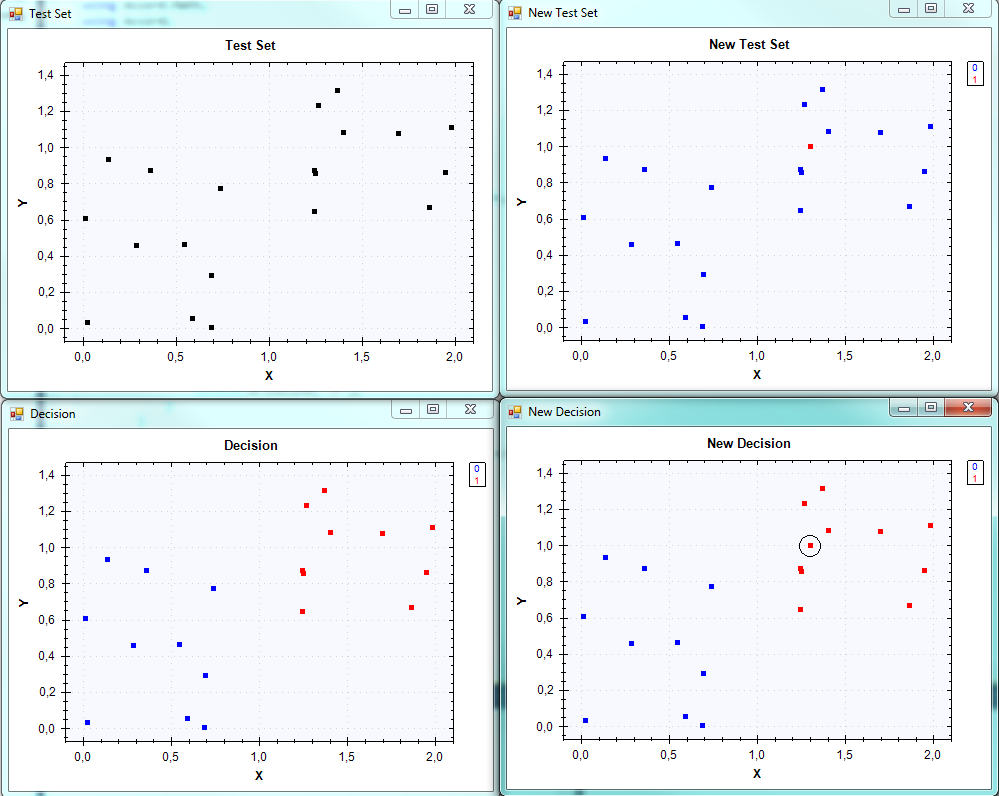
Here is an example with a test set that is easy to classify. The code is quite self explanatory with what we have said so far. We generate a set that is quite easy to classify. In the varialbe new_test_set we have added a new point (in red in the top right figure). We then make a new prediction and, since the point is on the top right, is correcly predicted as being part of the “red” class, +1.

If we print the variable new_prediction that gives us the predicted label of new_test_point we get +1 (or True) as it should.

using Accord.Controls;
using Accord.MachineLearning.VectorMachines.Learning;
using Accord.Math.Optimization.Losses;
using Accord.Statistics;
using Accord.Statistics.Kernels;
using Accord.Math;
using Accord;
using System;
using System.Linq;
using System.Windows.Forms;
using System.Collections.Generic;


namespace ConsoleApplication1
{
    class Program
    {
        public static void PrintJaggedMatrix<T>(T[][] matrix, string message = null)
        {
            Console.WriteLine(message);
            int i = 0;
            foreach (T[] col in matrix)
            {
                Console.WriteLine("Row {0}", i+1);
                i += 1;
                foreach (T row in col)
                {
                    Console.Write("{0:N5}\t", row);
                }
                Console.WriteLine("\n");
            }
        }

        public static void PrintArray<T>(T[] array, string message = null)
        {
            Console.WriteLine(message);
            int i = 0;    
            foreach (T item in array)
            {
                Console.WriteLine("{0:N5}", item);
            }
        }

        static void Main(string[] args)
        {
            // Test set. Generate a Nx2 random array
            // To make it easy generate 2 sets far apart.
            // Easy Linear SVM classification Example

            // number of points in the dataset
            int n_points = 10;
            // first set of points
            var x1 = Accord.Math.Jagged.Random(n_points, 1, 0.0, 1.1);
            var y1 = Accord.Math.Jagged.Random(n_points, 1, 0.0, 1.0);
            var set1 = Accord.Math.Matrix.Concatenate(x1, y1);
            set1 = set1.Transpose();
            //PrintJaggedMatrix(set1.Transpose(), "set1:\n");// Print the first set

            // second set of points
            var x2 = Accord.Math.Jagged.Random(n_points, 1, 1.1, 2.0);
            var y2 = Accord.Math.Jagged.Random(n_points, 1, 0.5, 1.5);
            var set2 = Accord.Math.Matrix.Concatenate(x2, y2);
            set2 = set2.Transpose();
            //PrintJaggedMatrix(set2.Transpose(),"set2:\n"); // Print the first set

            // Test Set
            var test_set = Accord.Math.Matrix.Concatenate(set1, set2).Transpose();

            // Print the Test Set
            //PrintJaggedMatrix(test_set, "Training Set:\n");

            // Plot the Test Set    
            ScatterplotBox.Show("Test Set", test_set);
            
            // Labels for the test set
            // Half of the test set is indexed -1 and half +1
            var labels1 = new int[10];
            var labels2 = new int[10];
            labels1.Set(-1, labels1.GetIndices());
            labels2.Set(1, labels2.GetIndices());
            var labels = Enumerable.ToArray(labels1.Concat(labels2));
            

            // Use the SMO algorithm to solve the quadratic optimization
            // Gaussian kernel for example
            var kernel = new Gaussian();
            // Create a pre-computed Gaussian kernel matrix
            var precomputed = new Precomputed(kernel.ToJagged(test_set));

            var minimizer = new SequentialMinimalOptimization<Precomputed, int>()
            {
                UseComplexityHeuristic = true,
                Kernel = precomputed
            };

            // define the SVM with the minimizer           
            var svm = minimizer.Learn(precomputed.Indices, labels);
            // Decisions predicted by the machine
            bool[] prediction = svm.Decide(precomputed.Indices);
            var answer = prediction.ToMinusOnePlusOne();
            ScatterplotBox.Show("Decision", test_set, answer);           
          

            // Add a new point (1.3, 1) to the test set and make a new decision
            double[][] new_test_point = { new double[] {1.3, 1.0}};
            // The new point is at the end of "test_set"
            var new_test_set = test_set.Transpose().Concatenate(new_test_point.Transpose()).Transpose();

            // Plot new Test Set
            var vec = Accord.Math.Vector.Zeros<int>(n_points*2+1); // vec is only there to color red new_test_point
            // Just for plotting
            vec[vec.Length - 1] = 1;
            ScatterplotBox.Show("New Test Set", new_test_set, vec);
            
            
            precomputed = new Precomputed(kernel.ToJagged2(test_set, new_test_point));
            svm.Kernel = precomputed;

            bool[] new_prediction = svm.Decide(precomputed.Indices);
            var new_answer = new_prediction.ToMinusOnePlusOne();

            // add new_answer to the known answers
            new_answer = answer.Concatenate(vec[vec.Length - 1]);      

            ScatterplotBox.Show("New Decision", new_test_set, new_answer);           

            //Console.ReadLine();          
        }

    }
}

png